【GluonTS】DeepARモデルとDeepFactorモデルとMQCNNモデルを比較してみる

はじめに

GluonTSのTSは「Time Series」の略です。GluonTSは時系列データを扱うツールになります。

いろいろな深層学習モデルが利用できるのですが今回はDeepARモデルとDeepFactorモデルとMQCNNモデルを使ってみます。
DeepARとDeepFactorはprobabilistic forecast、MQCNNはquantile forecastに分類されていますが適切な日本語訳がわかりませんしその違いも不明です。


いずれも過去の時系列データをもとに将来の値を推測するモデルです。

GluonTSで扱う時の三つの違い

GluonTSを使うと三つのモデルがほとんど同じスクリプトで実行できます。
ただし戻り値のクラスが異なります。

スクリプト内に注釈を入れていますがDeepARとDeepFactorの戻り値は「gluonts.model.forecast.SampleForecast」クラス、MQCNNの戻り値は「gluonts.model.forecast.QuantileForecast」クラスです。

そのためかプロットした時の結果はずいぶん異なる印象です。

結果

先にそれぞれの結果を示します。

DeepARの結果

DeepFactorの結果

MQCNNの結果

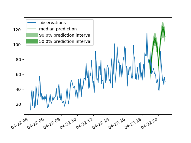
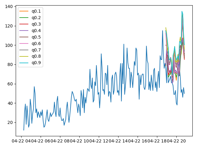
今回はとりあえず動かすことが目標ですのでパラメーターの設定は適当です。epochも10と非常に少ないです。
今回の結果だけでどのモデルが優れているとかの判断はできません。

Pythonスクリプト

DeepARモデル

from gluonts.dataset import common
from gluonts.model.deepar import DeepAREstimator
from gluonts.mx.trainer import Trainer
from gluonts.evaluation.backtest import make_evaluation_predictions

import pandas as pd
from matplotlib import pyplot as plt

url = "https://raw.githubusercontent.com/numenta/NAB/master/data/realTweets/Twitter_volume_AMZN.csv"
df = pd.read_csv(url, header=0, index_col=0)

train_data = common.ListDataset([{
    "start": df.index[0],
    "target": df.value[:-24]
    }],
    freq="5min")

test_data = common.ListDataset([{
    "start": df.index[0],
    "target": df.value
    }],
    freq="5min")

estimator = DeepAREstimator(
    freq = "5min", 
    prediction_length = 24, 
    context_length = 24,
    trainer = Trainer(epochs = 10))

predictor = estimator.train(train_data)

forecast_it, ts_it = make_evaluation_predictions(
    dataset=test_data,      # test dataset
    predictor=predictor,    # predictor
    num_samples=100,        # number of sample paths we want for evaluation
)

forecast = next(iter(forecast_it))  #<class 'gluonts.model.forecast.SampleForecast'>
ts = next(iter(ts_it))              #<class 'pandas.core.frame.DataFrame'>

prediction_intervals = (50.0, 90.0)
legend = ["observations", "median prediction"] + [f"{k}% prediction interval" for k in prediction_intervals][::-1]

plt.plot(ts[-200:])
forecast.plot(color='g', prediction_intervals=prediction_intervals)
plt.legend(legend, loc='upper left')

plt.show()

DeepFactorモデル

from gluonts.dataset import common
from gluonts.model.deep_factor import DeepFactorEstimator
from gluonts.mx.trainer import Trainer
from gluonts.evaluation.backtest import make_evaluation_predictions

import pandas as pd
from matplotlib import pyplot as plt

url = "https://raw.githubusercontent.com/numenta/NAB/master/data/realTweets/Twitter_volume_AMZN.csv"
df = pd.read_csv(url, header=0, index_col=0)

train_data = common.ListDataset([{
    "start": df.index[0],
    "target": df.value[:-24]
    }],
    freq="5min")

test_data = common.ListDataset([{
    "start": df.index[0],
    "target": df.value
    }],
    freq="5min")

estimator = DeepFactorEstimator(
    freq = "5min", 
    prediction_length = 24, 
    context_length = 24,
    trainer = Trainer(epochs = 10))

predictor = estimator.train(train_data)

forecast_it, ts_it = make_evaluation_predictions(
    dataset=test_data,      # test dataset
    predictor=predictor,    # predictor
    num_samples=100,        # number of sample paths we want for evaluation
)

forecast = next(iter(forecast_it))  #<class 'gluonts.model.forecast.SampleForecast'>
ts = next(iter(ts_it))              #<class 'pandas.core.frame.DataFrame'>

prediction_intervals = (50.0, 90.0)
legend = ["observations", "median prediction"] + [f"{k}% prediction interval" for k in prediction_intervals][::-1]

plt.plot(ts[-200:])
forecast.plot(color='g', prediction_intervals=prediction_intervals)
plt.legend(legend, loc='upper left')

plt.show()

MQCNNモデル

from gluonts.dataset import common
from gluonts.model.seq2seq import MQCNNEstimator
from gluonts.mx.trainer import Trainer
from gluonts.evaluation import make_evaluation_predictions

import pandas as pd
from matplotlib import pyplot as plt

url = "https://raw.githubusercontent.com/numenta/NAB/master/data/realTweets/Twitter_volume_AMZN.csv"
df = pd.read_csv(url, header=0, index_col=0)

train_data = common.ListDataset([{
    "start": df.index[0],
    "target": df.value[:-24]
    }],
    freq="5min")

test_data = common.ListDataset([{
    "start": df.index[0],
    "target": df.value
    }],
    freq="5min")

estimator = MQCNNEstimator(
    freq = "5min",
    prediction_length = 24,
    context_length = 24,
    trainer = Trainer(epochs = 10))

predictor = estimator.train(train_data)

forecast_it, ts_it = make_evaluation_predictions(
    dataset=test_data,      # test dataset
    predictor=predictor,    # predictor
    num_samples=100,        # number of sample paths we want for evaluation
)

forecast = next(iter(forecast_it))  #<class 'gluonts.model.forecast.QuantileForecast'>
ts = next(iter(ts_it))              #<class 'pandas.core.frame.DataFrame'>

plt.plot(ts[-200:])
forecast.plot()

plt.tight_layout()

plt.show()

GluonTSを使うための環境構築

pip install mxnet -f https://dist.mxnet.io/python/cpu
pip install gluonts

さいごに

MXNetをやめてPyTorchにのりかえたのですがまたMXNetに戻ってきました。

時系列データを扱うのに「pytorch-ts」というのもありますが今のところ開発で先行しているのは「GluonTS」です。そのうち逆転されるのでしょうけども・・・。

間違いや改善点があればコメント頂けましたら幸いです。