はじめに
文章を固定長のベクトルで表現することにチャレンジしました。
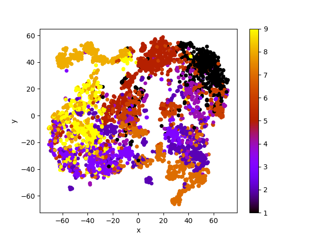
最後にt-SNEで2次元に落とし込んで図示しています。
使用するデータ
「livedoor ニュースコーパス」を使用させて頂く。
「ldcc-20140209.tar.gz」をダウンロードして「ldcc-20140209.tar」に名前を変更して解凍する。
tar xvf ldcc-20140209.tar
「text」フォルダが作成され、さらにその中に「dokujo-tsushin」「it-life-hack」「kaden-channel」「livedoor-homme」「movie-enter」「peachy」「smax」「sports-watch」「topic-news」の9個のフォルダが作成される。
それぞれのフォルダ内には各記事のデータが含まれるテキストファイルが入っている。
また、それぞれのフォルダ内に「LICENSE.txt」というテキストファイルも含まれる。開いて読んだのちに今回はファルダ外の任意の場所に移動させる。
ファイルの読み込み
1行目、2行目は記事のURL、日付なので3行目から読み込む。
with open("dokujo-tsushin\dokujo-tsushin-6877711.txt", encoding="utf-8_sig") as f:
    next(f)
    next(f)
    #全角スペースや改行の削除
    w = f.read().replace('\u3000','').replace('\n','')
または
with open("dokujo-tsushin\dokujo-tsushin-6877711.txt", encoding="utf-8_sig") as f:
    a = f.readlines()
    aa = ''.join(a[2:])
    #全角スペースや改行の削除
    w = aa.replace('\u3000','').replace('\n','')
下のほうがわずかに速い。
形態素解析と単語のID化→その後保存
形態素解析は「Janome」ライブラリを使用。(pipでインストール可能)
「Janome」と「MeCab」の違いは公式ページに記載あり。
解析結果の精度は。
辞書,言語モデルともに MeCab のデフォルトシステム辞書をそのまま使わせていただいているため,バグがなければ,MeCab と同等の解析結果になると思います。
形態素解析の速度は。
文章の長さによりますが,手元の PC では 1 センテンスあたり数ミリ〜数十ミリ秒でした。mecab-python の10倍程度(長い文章だとそれ以上)遅い,というくらいでしょうか。今のところは,大量の文書を高速にバッチ処理する用途には向いていません。MeCab をお使いください。
インストールが簡単なので「Janome」を選択した。
単語のID化は「collections」の「Counter」を使用。
import glob
import os
from collections import Counter
from janome.tokenizer import Tokenizer

tk = Tokenizer()
freq = Counter()

category = []   #カテゴリー
news_txt = []   #記事

for fn in glob.glob('*/*.txt'):
    (dirname,filename)=os.path.split(fn)

    with open(fn, encoding="utf-8_sig") as f:
        a = f.readlines()
        aa = ''.join(a[2:])
        #全角スペースや改行の削除
        w = aa.replace('\u3000','').replace('\n','')

    t = tk.tokenize(w)
    l = [p.surface for p in t]

    freq.update(set(l))
    category.append(dirname)
    news_txt.append(l)

#単語IDを出現回数の順に並べる(collections.Counterからlistに変換される)
common = freq.most_common()

#最小出現回数
min_df = 10

#最大出現回数
max_df = int(common[0][1] * 0.3)

#辞書を作成
vocab = sorted([t for t, c in common if c>=min_df and c < max_df])
index = {t:i+1 for i,t in enumerate(vocab)}

#学習用データと評価用データに分ける
from sklearn.model_selection import train_test_split
X_train, X_test, Y_train, Y_test = train_test_split(news_txt, category, test_size=0.3)

#データをcsvで保存する(ヘッダーなし)
termc = max(index.values()) + 1

with open('train.csv', 'w') as f:
    for i in range(len(X_train)):
        t = X_train[i]
        #辞書から単語IDのリストにする
        v = [index[c] for c in t if c in index]
        #リストの長さを250にそろえる
        if(len(v)<250):
            w = v + [termc] * int(250 - len(v))
        else:
            w = v[:250]
        f.write(Y_train[i])
        f.write(',')
        f.write(','.join(list(map(str,w))))
        f.write('\n')

with open('test.csv', 'w') as f:
    for i in range(len(X_test)):
        t = X_test[i]
        #辞書から単語IDのリストにする
        v = [index[c] for c in t if c in index]
        #リストの長さを250にそろえる
        if(len(v)<250):
            w = v + [termc] * int(250 - len(v))
        else:
            w = v[:250]
        f.write(Y_test[i])
        f.write(',')
        f.write(','.join(list(map(str,w))))
        f.write('\n')
モデルの作成
GRUを使用する
「gru.py」として保存
import mxnet as mx
from mxnet.gluon import Block, nn, rnn

ctx = mx.gpu()
#cpu = mx.cup()

class Model(Block):
    def __init__(self, word_num, hidden_size, **kwargs):
        super(Model, self).__init__(**kwargs)
        self.word_num = word_num
        self.hidden_size = hidden_size

        with self.name_scope():
            self.embed = nn.Embedding(word_num, hidden_size)
            self.rnn = rnn.GRU(hidden_size, num_layers=1)
            self.dense = nn.Dense(word_num, flatten=False)

    def forward(self, x):
        batch_size = x.shape[0]
        x = self.embed(x)
        x = mx.nd.swapaxes(x, 0, 1)
        h = mx.nd.random.uniform(shape=(1, batch_size, self.hidden_size),ctx=ctx)
        x, h = self.rnn(x, h)
        x = mx.nd.swapaxes(x, 0, 1)
        x = self.dense(x)
        return x, h
実行
import pandas as pd
import numpy as np

#データの読みこみ
df = pd.read_csv('train.csv', header=None)

#2番目以降の列が文章、最初の列がカテゴリー
words = df.iloc[:,1:].values

#逆順の文
X = [np.flip(x, axis=0) for x in words]

import mxnet as mx

ctx = mx.gpu()
#ctx = mx.cpu()

X = mx.nd.array(X)
Y = mx.nd.array(words)

from mxnet import autograd
from mxnet.gluon import Trainer
from mxnet.gluon.loss import SoftmaxCrossEntropyLoss
import gru

#モデルの作成
word_num = np.amax(words)
model = gru.Model(word_num, 128)
model.initialize(ctx=ctx)

#学習アルゴリズムの設定
trainer = Trainer(model.collect_params(), 'adam')
loss_func = SoftmaxCrossEntropyLoss()

#データの準備
train_data = mx.io.NDArrayIter(X, Y, batch_size=15, shuffle=True)

#学習の開始
print('start training...')

epochs = 30
loss_n = []

for i in range(1, epochs+1):
    train_data.reset()
    for batch in train_data:
        data = batch.data[0].as_in_context(ctx)
        label = batch.label[0].as_in_context(ctx)
        with autograd.record():
            output, status = model(data)
            loss = loss_func(output, label)
            loss_n.append(np.mean(loss.asnumpy()))
            loss.backward()
        trainer.step(batch.data[0].shape[0])

    ll = np.mean(loss_n)
    print('%d epoch  loss = %f'%(i, ll))
    loss_n = []

model.save_parameters('rnn_model.params')
結果の確認
import pandas as pd
import numpy as np

#データの読みこみ
df = pd.read_csv('train.csv', header=None)

#2番目以降の列が文章、最初の列がカテゴリー
words = df.iloc[:,1:].values
category = df.iloc[:,0].values

#カテゴリーを文字列からIDにする
category_dict = {t:i+1 for i,t in enumerate(np.unique(category))}
category =  [category_dict[c] for c in category]

#逆順の文
X = [np.flip(x, axis=0) for x in words]

import mxnet as mx

ctx = mx.gpu()
#ctx = mx.cpu()

X = mx.nd.array(X).as_in_context(ctx)

#モデルのインポート
import gru
word_num = np.amax(words)
model = gru.Model(word_num, 128)
model.load_parameters('rnn_model.params', ctx=ctx)

#モデルの実行
output, status = model(X)

#ステータスの取得
doc_vec = status[0].asnumpy()[0]

#t-SNEで2次元に
from sklearn.manifold import TSNE
result = TSNE(n_components=2, random_state=0).fit_transform(doc_vec)

#結果を散布図にして表示
import matplotlib.pyplot as plt
df_plot = pd.DataFrame({'x':result[:,0], 'y':result[:,1], 'c':category})
df_plot.plot(kind='scatter', x='x', y='y', c=category, colormap='gnuplot')
plt.show()
参考文献

- 作者:坂本 俊之
- 発売日: 2018/06/26
- メディア: 単行本(ソフトカバー)